Error Bars

This example teaches you how to add error bars to a chart in Excel.

1. Select the chart.

2. Click the + button on the right side of the chart, click the arrow next to Error Bars and then click More Options.



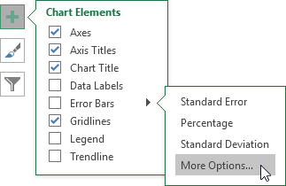
Notice the shortcuts to quickly display error bars using the Standard Error, a percentage value of 5% or 1 standard deviation.

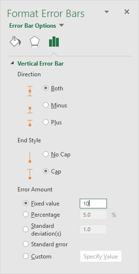
The Format Error Bars pane appears.

3. Choose a Direction. Click Both.

4. Choose an End Style. Click Cap.

5. Click Fixed value and enter the value 10.



Result:



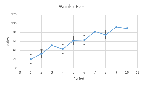
Note: if you add error bars to a scatter chart, Excel also adds horizontal error bars. In this example, these error bars have been removed..