DW Faisalabad New Version

DW Faisalabad New Version
Please Jump to New Version
Showing posts with label Analysis ToolPak. Show all posts

Sunday, 9 July 2017

Regression

R Square  |  Significance F and P-Values  |  Coefficients  |  Residuals

This example teaches you how to perform a regression analysis in Excel and how to interpret the Summary Output.

Below you can find our data. The big question is: is there a relation between Quantity Sold (Output) and Price and Advertising (Input). In other words: can we predict Quantity Sold if we know Price and Advertising?


1. On the Data tab, in the Analysis group, click Data Analysis.


Note: can't find the Data Analysis button? Click here to load the Analysis ToolPak add-in.

2. Select Regression and click OK.


3. Select the Y Range (A1:A8). This is the predictor variable (also called dependent variable).

4. Select the X Range(B1:C8). These are the explanatory variables (also called independent variables). These columns must be adjacent to each other.

5. Check Labels.

6. Click in the Output Range box and select cell A11.

7. Check Residuals.

8. Click OK.


Excel produces the following Summary Output (rounded to 3 decimal places).

R Square

R Square equals 0.962, which is a very good fit. 96% of the variation in Quantity Sold is explained by the independent variables Price and Advertising. The closer to 1, the better the regression line (read on) fits the data.


Significance F and P-values

To check if your results are reliable (statistically significant), look at Significance F (0.001). If this value is less than 0.05, you're OK. If Significance F is greater than 0.05, it's probably better to stop using this set of independent variables. Delete a variable with a high P-value (greater than 0.05) and rerun the regression until Significance F drops below 0.05.

Most or all P-values should be below below 0.05. In our example this is the case. (0.000, 0.001 and 0.005).


Coefficients

The regression line is: y = Quantity Sold = 8536.214 -835.722 * Price + 0.592 * Advertising. In other words, for each unit increase in price, Quantity Sold decreases with 835.722 units. For each unit increase in Advertising, Quantity Sold increases with 0.592 units. This is valuable information.

You can also use these coefficients to do a forecast. For example, if price equals $4 and Advertising equals $3000, you might be able to achieve a Quantity Sold of 8536.214 -835.722 * 4 + 0.592 * 3000 = 6970.

Residuals

The residuals show you how far away the actual data points are fom the predicted data points (using the equation). For example, the first data point equals 8500. Using the equation, the predicted data point equals 8536.214 -835.722 * 2 + 0.592 * 2800 = 8523.009, giving a residual of 8500 - 8523.009 = -23.009.


You can also create a scatter plot of these residuals.

.
Read More »

Correlation

The correlation coefficient (a value between -1 and +1) tells you how strongly two variables are related to each other. We can use the CORREL function or the Analysis Toolpak add-in in Excel to find the correlation coefficient between two variables.

- A correlation coefficient of +1 indicates a perfect positive correlation. As variable X increases, variable Y increases. As variable X decreases, variable Y decreases.


- A correlation coefficient of -1 indicates a perfect negative correlation. As variable X increases, variable Z decreases. As variable X decreases, variable Z increases.


- A correlation coefficient near 0 indicates no correlation.

To use the Analysis Toolpak add-in in Excel to quickly generate correlation coefficients between multiple variables, execute the following steps.

1. On the Data tab, in the Analysis group, click Data Analysis.


Note: can't find the Data Analysis button? Click here to load the Analysis ToolPak add-in.

2. Select Correlation and click OK.


3. For example, select the range A1:C6 as the Input Range.


4. Check Labels in first row.

5. Select cell A8 as the Output Range.

6. Click OK.


Result.


Conclusion: variables A and C are positively correlated (0.91). Variables A and B are not correlated (0.19). Variables B and C are also not correlated (0.11) . You can verify these conclusions by looking at the graph..
Read More »

Exponential Smoothing

This example teaches you how to apply exponential smoothing to a time series in Excel. Exponential smoothing is used to smooth out irregularities (peaks and valleys) to easily recognize trends.

1. First, let's take a look at our time series.


2. On the Data tab, in the Analysis group, click Data Analysis.


Note: can't find the Data Analysis button? Click here to load the Analysis ToolPak add-in.

3. Select Exponential Smoothing and click OK.


4. Click in the Input Range box and select the range B2:M2.

5. Click in the Damping factor box and type 0.9. Literature often talks about the smoothing constant α (alpha). The value (1- α) is called the damping factor.

6. Click in the Output Range box and select cell B3.

7. Click OK.


8. Plot a graph of these values.


Explanation: because we set alpha to 0.1, the previous data point is given a relatively small weight while the previous smoothed value is given a large weight (i.e. 0.9). As a result, peaks and valleys are smoothed out. The graph shows an increasing trend. Excel cannot calculate the smoothed value for the first data point because there is no previous data point. The smoothed value for the second data point equals the previous data point.

9. Repeat steps 2 to 8 for alpha = 0.3 and alpha = 0.8.


Conclusion: The smaller alpha (larger the damping factor), the more the peaks and valleys are smoothed out. The larger alpha (smaller the damping factor), the closer the smoothed values are to the actual data points..
Read More »

Moving Average

This example teaches you how to calculate the moving average of a time series in Excel. A moving average is used to smooth out irregularities (peaks and valleys) to easily recognize trends.

1. First, let's take a look at our time series.


2. On the Data tab, in the Analysis group, click Data Analysis.


Note: can't find the Data Analysis button? Click here to load the Analysis ToolPak add-in.

3. Select Moving Average and click OK.


4. Click in the Input Range box and select the range B2:M2.

5. Click in the Interval box and type 6.

6. Click in the Output Range box and select cell B3.

7. Click OK.


8. Plot a graph of these values.


Explanation: because we set the interval to 6, the moving average is the average of the previous 5 data points and the current data point. As a result, peaks and valleys are smoothed out. The graph shows an increasing trend. Excel cannot calculate the moving average for the first 5 data points because there are not enough previous data points.

9. Repeat steps 2 to 8 for interval = 2 and interval = 4.


Conclusion: The larger the interval, the more the peaks and valleys are smoothed out. The smaller the interval, the closer the moving averages are to the actual data points..
Read More »

t-Test

This example teaches you how to perform a t-Test in Excel. The t-Test is used to test the null hypothesis that the means of two populations are equal.

Below you can find the study hours of 6 female students and 5 male students.


To perform a t-Test, execute the following steps.

1. First, perform an F-Test to determine if the variances of the two populations are equal. This is not the case.

2. On the Data tab, in the Analysis group, click Data Analysis.


Note: can't find the Data Analysis button? Click here to load the Analysis ToolPak add-in.

3. Select t-Test: Two-Sample Assuming Unequal Variances and click OK.


4. Click in the Variable 1 Range box and select the range A2:A7.

5. Click in the Variable 2 Range box and select the range B2:B6.

6. Click in the Hypothesized Mean Difference box and type 0 (H0: μ1 - μ2 = 0).

7. Click in the Output Range box and select cell E1.


8. Click OK.

Result:


Conclusion: We do a two-tail test (inequality). lf t Stat < -t Critical two-tail or t Stat > t Critical two-tail, we reject the null hypothesis. This is not the case, -2.365 < 1.473 < 2.365. Therefore, we do not reject the null hypothesis. The observed difference between the sample means (33 - 24.8) is not convincing enough to say that the average number of study hours between female and male students differ significantly..
Read More »

F-Test

This example teaches you how to perform an F-Test in Excel. The F-Test is used to test the null hypothesis that the variances of two populations are equal.

Below you can find the study hours of 6 female students and 5 male students.


To perform an F-Test, execute the following steps.

1. On the Data tab, in the Analysis group, click Data Analysis.


Note: can't find the Data Analysis button? Click here to load the Analysis ToolPak add-in.

2. Select F-Test Two-Sample for Variances and click OK.


3. Click in the Variable 1 Range box and select the range A2:A7.

4. Click in the Variable 2 Range box and select the range B2:B6.

5. Click in the Output Range box and select cell E1.


6. Click OK.

Result:


Important: be sure that the variance of Variable 1 is higher than the variance of Variable 2. This is the case, 160 > 21.7. If not, swap your data. As a result, Excel calculates the correct F value, which is the ratio of Variance 1 to Variance 2 (F = 160 / 21.7 = 7.373).

Conclusion: if F > F Critical one-tail, we reject the null hypothesis. This is the case, 7.373 > 6.256. Therefore, we reject the null hypothesis. The variances of the two populations are unequal..
Read More »

Anova

This example teaches you how to perform a single factor ANOVA (analysis of variance) in Excel. A single factor or one-way ANOVA is used to test the null hypothesis that the means of several populations are all equal.

Below you can find the salaries of people who have a degree in economics, medicine or history.


To perform a single factor ANOVA, execute the following steps.

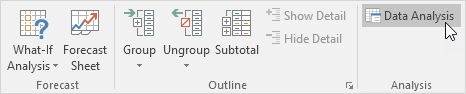
1. On the Data tab, in the Analysis group, click Data Analysis.


Note: can't find the Data Analysis button? Click here to load the Analysis ToolPak add-in.

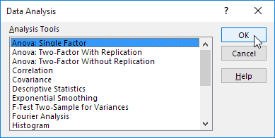
2. Select Anova: Single Factor and click OK.


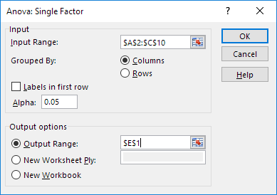
3. Click in the Input Range box and select the range A2:C10.

4. Click in the Output Range box and select cell E1.


5. Click OK.

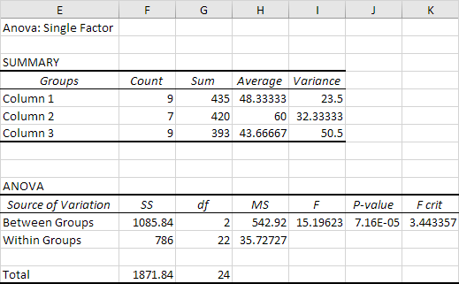
Result:


Conclusion: if F > F crit, we reject the null hypothesis. This is the case, 15.196 > 3.443. Therefore, we reject the null hypothesis. The means of the three populations are not all equal. At least one of the means is different. However, the ANOVA does not tell you where the difference lies. You need a t-Test to test each pair of means..
Read More »

Descriptive Statistics

You can use the Analysis Toolpak add-in to generate descriptive statistics. For example, you may have the scores of 14 participants for a test.


To generate descriptive statistics for these scores, execute the following steps.

1. On the Data tab, in the Analysis group, click Data Analysis.


Note: can't find the Data Analysis button? Click here to load the Analysis ToolPak add-in.

2. Select Descriptive Statistics and click OK.


3. Select the range A2:A15 as the Input Range.

4. Select cell C1 as the Output Range.

5. Make sure Summary statistics is checked.


6. Click OK.

Result:

.
Read More »