Digital World Faisalabad: Array Formulas

Showing posts with label Array Formulas. Show all posts

Monday, 3 July 2017

System of Linear Equations

This example shows you how to solve a system of linear equations in Excel. For example, we have the following system of linear equations:

If A^-1 (the inverse of A) exists, we can multiply both sides by A-1 to obtain X = A-1B. To solve this system of linear equations in Excel, execute the following steps.

1. Use the MINVERSE function to return the inverse matrix of A. First, select the range B6:D8. Next, insert the MINVERSE function shown below. Finish by pressing CTRL + SHIFT + ENTER.

Note: the formula bar indicates that the cells contain an array formula. Therefore, you cannot delete a single result. To delete the results, select the range B6:D8 and press Delete.

2. Use the MMULT function to return the product of matrix A-1 and B. First, select the range G6:G8. Next, insert the MMULT function shown below. Finish by pressing CTRL + SHIFT + ENTER.

3. Put it all together. First, select the range G6:G8. Next, insert the formula shown below. Finish by pressing CTRL + SHIFT + ENTER.

Most Frequently Occurring Word

This example teaches you how to find the most frequently occurring word in Excel.

You can use the MODE function to find the most frequently occurring number. However, the MODE function only works with numbers.

You can use the COUNTIF function to count the number of occurrences of each word. However, we are looking for a single formula that returns the most frequently occurring word (circle in our example).

To find the most frequently occurring word, execute the following steps.

1. The MATCH function returns the position of a value in a given range.

Explanation: circle (A7) found at position 2 in the range A1:A7. Set the third argument to 0 to return an exact match.

2. To find the position of the most frequently occurring word (don't be overwhelmed), we add the MODE function and replace A7 with A1:A7.

3. Finish by pressing CTRL + SHIFT + ENTER.

Note: The formula bar indicates that this is an array formula by enclosing it in curly braces {}. Do not type these yourself. They will disappear when you edit the formula.

Explanation: The range (array constant) created by the MATCH function is stored in Excel's memory, not in a range. The array constant looks as follows:

{1;2;2;2;5;5;2} - (triangle found at position 1, circle found at position 2, circle found at position 2, etc.)

This array constant is used as an argument for the MODE function, giving a result of 2 (the position of the most frequently occurring word).

4. Use this result and the INDEX function to return the 2nd word in the range A1:A7, the most frequently occurring word.

Two-column Lookup

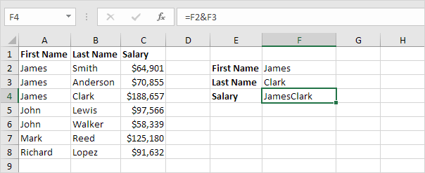
This example teaches you how to perform a two-column lookup in Excel. See the example below. We want to look up the salary of James Clark, not James Smith, not James Anderson.

1. To join strings, use the & operator.

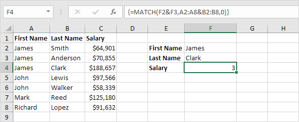
2. The MATCH function returns the position of a value in a given range. Insert the MATCH function shown below.

3. Finish by pressing CTRL + SHIFT + ENTER.

Note: The formula bar indicates that this is an array formula by enclosing it in curly braces {}. Do not type these yourself. They will disappear when you edit the formula.

Explanation: The range (array constant) A2:A8&B2:B8 is stored in Excel's memory, not in a range. The array constant looks as follows:

{"JamesSmith";"JamesAnderson";"JamesClark";"JohnLewis";"JohnWalker";"MarkReed";"RichardLopez"}

This array constant is used as an argument for the MATCH function, giving a result of 3 (JamesClark found at position 3).

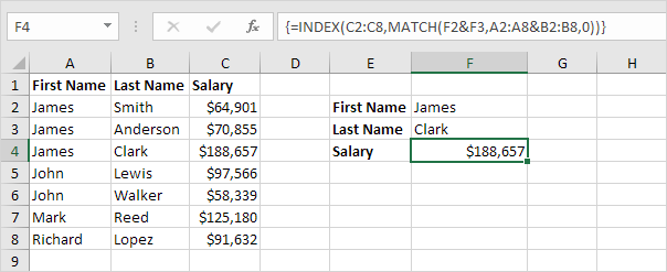
4. Use this result and the INDEX function to return the 3rd value in the range C2:C8.

Sum with Or Criteria

Summing with Or criteria in Excel can be tricky. This article shows several easy to follow examples.

1. We start simple. For example, we want to sum the cells that meet the following criteria: Google or Facebook (one criteria range).

2a. However, if we want to sum the cells that meet the following criteria: Google or Stanford (two criteria ranges), we cannot simply use the SUMIF function twice (see the picture below). Cells that meet the criteria Google and Stanford are added twice, but they should only be added once. 10 is the answer we are looking for.

2b. We need an array formula. We use the IF function to check if Google or Stanford occurs.

Explanation: TRUE = 1, FALSE = 0. For row 1, the IF function evaluates to IF(TRUE+TRUE,1,0)*3, IF(2,1,0)*3, 3. So the value 3 will be added. For row 2, the IF function evaluates to IF(FALSE+FALSE,1,0)*5, IF(0,1,0)*5, 0. So the value 5 will not be added. For row 3, the IF function evaluates to IF(FALSE+TRUE,1,0)*2, IF(1,1,0)*2, 2. So the value 2 will be added, etc.

2c. All we need is a SUM function that sums these values. To achieve this (don't be overwhelmed), we add the SUM function and replace A1 with A1:A8, B1 with B1:B8 and C1 with C1:C8.

2d. Finish by pressing CTRL + SHIFT + ENTER.

Note: The formula bar indicates that this is an array formula by enclosing it in curly braces {}. Do not type these yourself. They will disappear when you edit the formula.

Explanation: The range (array constant) created by the IF function is stored in Excel's memory, not in a range. The array constant looks as follows:

{1;0;1;0;1;0;1;0}

multiplied by C1:C8 this yields:

{3;0;2;0;4;0;1;0}

This latter array constant is used as an argument for the SUM function, giving a result of 10.

3. We can go one step further. For example, we want to sum the cells that meet the following criteria: (Google and Stanford) or Columbia.

Sum Range with Errors

This example shows you how to create an array formula that sums a range with errors. You can also use the AGGREGATE function to sum a range with errors.

1. We use the IFERROR function to check for an error.

Explanation: the IFERROR function returns 0, if an error is found. If not, it returns the value of the cell.

2. To sum the range with errors (don't be overwhelmed), we add the SUM function and replace A1 with A1:A7.

3. Finish by pressing CTRL + SHIFT + ENTER.

Sum Largest Numbers

This example shows you how to create an array formula that sums the largest numbers in a range.

1. We use the LARGE function. For example, to find the second to largest number, use the following function.

2. To sum the 4 largest numbers (don't be overwhelmed), add the SUM function and replace 2 with {1,2,3,4}.

3. Finish by pressing CTRL + SHIFT + ENTER.

Sum Every nth Row

This example shows you how to create an array formula that sums every nth row in Excel. We will show it for n = 3, but you can do this for any number.

1. The ROW function returns the row number of a cell.

2. The MOD function gives the remainder of a division. For example, for the first row, MOD(1,3) equals 1. 1 is divided by 3 (0 times) to give a remainder of 1. For the third row, MOD(3,3) equals 0. 3 is divided by 3 (exactly 1 time) to give a remainder of 0. As a result, the formula returns 0 for every 3th row.

Note: change the 3 to 4 to sum every 4th row, to 5 to sum every 5th row, etc.

3. Slightly change the formula as shown below.

4. To get the sum of the product of these two ranges (FALSE=0, TRUE=1), use the SUM function and finish by pressing CTRL + SHIFT + ENTER.

Count with Or Criteria

Counting with Or criteria in Excel can be tricky. This article shows several easy to follow examples.

1. We start simple. For example, we want to count the number of cells that contain Google or Facebook (one column).

2a. However, if we want to count the number of rows that contain Google or Stanford (two columns), we cannot simply use the COUNTIF function twice (see the picture below). Rows that contain Google and Stanford are counted twice, but they should only be counted once. 4 is the answer we are looking for.

2b. What we need is an array formula. We use the IF function to check if Google or Stanford occurs.

Explanation: TRUE = 1, FALSE = 0. For row 1, the IF function evaluates to IF(TRUE+TRUE,1,0), IF(2,1,0), 1. So the first row will be counted. For row 2, the IF function evaluates to IF(FALSE+FALSE,1,0), IF(0,1,0), 0. So the second row will not be counted. For row 3, the IF function evaluates to IF(FALSE+TRUE,1,0), IF(1,1,0), 1. So the third row will be counted, etc.

2c. All we need is a SUM function that counts these 1's. To achieve this (don't be overwhelmed), we add the SUM function and replace A1 with A1:A8 and B1 with B1:B8.

2d. Finish by pressing CTRL + SHIFT + ENTER.

Note: The formula bar indicates that this is an array formula by enclosing it in curly braces {}. Do not type these yourself. They will disappear when you edit the formula.

Explanation: The range (array constant) created by the IF function is stored in Excel's memory, not in a range. The array constant looks as follows:

{1;0;1;0;1;0;1;0}

This array constant is used as an argument for the SUM function, giving a result of 4.

3. We can go one step further. For example, we want to count the number of rows that contain (Google and Stanford) or Columbia.

Count Unique Values

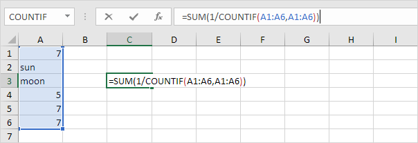
This example shows you how to create an array formula that counts unique values.

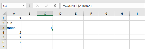
1. We use the COUNTIF function. For example, to count the number of 5's, use the following function.

2. To count the unique values (don't be overwhelmed), we add the SUM function, 1/, and replace 5 with A1:A6.

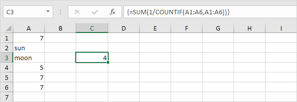
3. Finish by pressing CTRL + SHIFT + ENTER.

Note: The formula bar indicates that this is an array formula by enclosing it in curly braces {}. Do not type these yourself. They will disappear when you edit the formula.

Explanation: The range (array constant) created by the COUNTIF function is stored in Excel's memory, not in a range. The array constant looks as follows:

{3;1;1;1;3;3} - (three 7's, one sun, one moon, one 5, three 7's, three 7's)

This reduces to:
{1/3;1/1;1/1;1/1;1/3;1/3}

This array constant is used as an argument for the SUM function, giving a result of 1/3+1+1+1+1/3+1/3 = 4..

Count Errors

This example shows you how to create an array formula that counts the number of errors in a range.

1. We use the IF function and the ISERROR function to check for an error.

Explanation: the IF function returns 1, if an error is found. If not, it returns an empty string.

2. To count the errors (don't be overwhelmed), we add the COUNT function and replace A1 with A1:C3.

3. Finish by pressing CTRL + SHIFT + ENTER.

Note: The formula bar indicates that this is an array formula by enclosing it in curly braces {}. Do not type these yourself. They will disappear when you edit the formula.

Explanation: The range (array constant) created by the IF function is stored in Excel's memory, not in a range. The array constant looks as follows:

{1,"",1;"","","";"","",1}

This array constant is used as an argument for the COUNT function, giving a result of 3.

4. To count specific errors, use the COUNTIF function. For example, to count the number of cells that contain the #DIV/0! error.

Array Formulas

Without Array Formula | With Array Formula | F9 Key

This chapter helps you understand array formulas in Excel. Single cell array formulas perform multiple calculations in one cell.

Without Array Formula

Without using an array formula, we would execute the following steps to find the greatest progress.

1. First, we would calculate the progress of each student.

2. Next, we would use the MAX function to find the greatest progress.

With Array Formula

We don't need to store the range in column D. Excel can store this range in its memory. A range stored in Excel's memory is called an array constant.

1. We already know that we can find the progress of the first student by using the formula below.

2. To find the greatest progress (don't be overwhelmed), we add the MAX function, replace C2 with C2:C6 and B2 with B2:B6.

3. Finish by pressing CTRL + SHIFT + ENTER.

Note: The formula bar indicates that this is an array formula by enclosing it in curly braces {}. Do not type these yourself. They will disappear when you edit the formula.

Explanation: The range (array constant) is stored in Excel's memory, not in a range. The array constant looks as follows:

{19;33;63;48;13}

This array constant is used as an argument for the MAX function, giving a result of 63.

F9 Key

When working with array formulas, you can have a look at these array constants yourself.

1. Select C2:C6-B2:B6 in the formula.

2. Press F9.

That looks good. Elements in a vertical array constant are separated by semicolons. Elements in a horizontal array constant are separated by commas..

DW Faisalabad New Version

Monday, 3 July 2017