Checklist

This example teaches you how to create a checklist in Excel. First, turn on the Developer tab. Next, you can create a checklist.



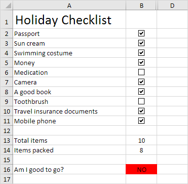
To create this checklist, execute the following steps.

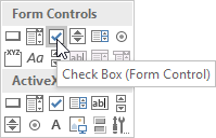
1. On the Developer tab, in the Controls group, click Insert.



2. Click Check Box in the Form Controls section.



3. Draw a check box in cell B2.



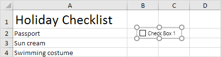
4. To remove "Check Box 1", right click the check box, click the text and delete it.

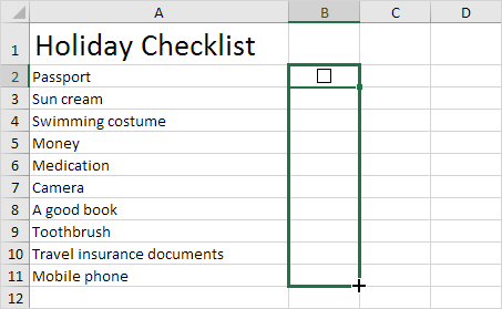
5. Select cell B2.

6. Click on the lower right corner of cell B2 and drag it down to cell B11.



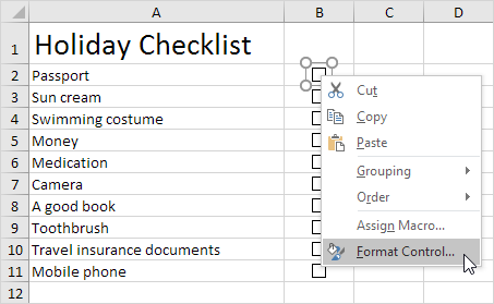
7. Right click the first check box and click Format Control.



8. Link the check box to the cell next to it (cell C2).



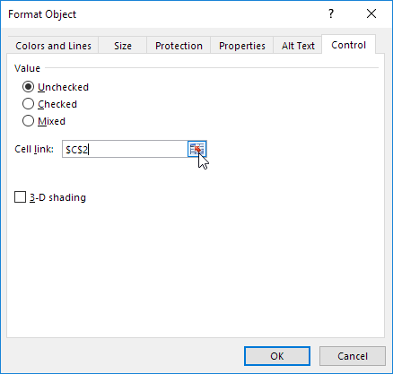
9. Repeat step 8 for the other check boxes.

10. The count the number of items packed, insert a COUNTIF function into cell B14.



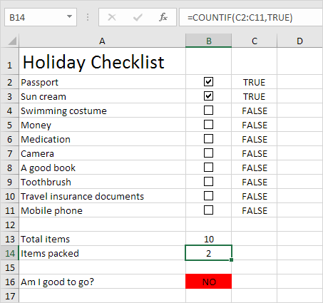
11. Hide column C.

12. Insert an IF function into cell B16.

Result:



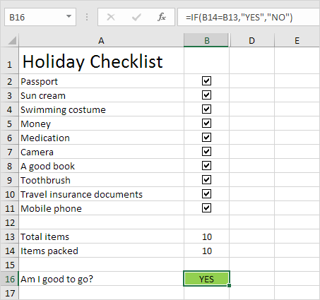
Note: we created a conditional formatting rule to change the background color of cell B16 depending on the cell's value..

Read More »

Conflicting Rules

Sometimes multiple conditional formatting rules in Excel conflict. A higher rule always wins. This example illustrates two different results.

1. The value 95 is higher than 80 but is also the highest value (Top 1). The formats (yellow fill vs green fill and yellow text color vs green text color) conflict. A higher rule always wins. As a result, the value 95 is colored yellow.



Result:



2. Move the second rule up. The value 95 is the highest value (Top 1) but is also higher than 80. The formats (green fill vs yellow fill and green text color vs yellow text color) conflict. A higher rule always wins. As a result, the value 95 is colored green.



Result:



Note: only use the Stop If True check boxes for backwards compatibility with earlier versions of Microsoft Excel..

Read More »

Compare Two Lists

This example describes how to compare two lists using conditional formatting. For example, you may have two lists of NFL teams.



To highlight the teams in the first list that are not in the second list, execute the following steps.

1. First, select the range A1:A18 and name it firstList, select the range B1:B20 and name it secondList.

2. Next, select the range A1:A18.

3. On the Home tab, in the Styles group, click Conditional Formatting.



4. Click New Rule.



5. Select 'Use a formula to determine which cells to format'.

6. Enter the formula =COUNTIF(secondList,A1)=0

7. Select a formatting style and click OK.



Result. Miami Dolphins and Tennessee Titans are not in the second list.



Explanation: =COUNTIF(secondList,A1) counts the number of teams in secondList that are equal to the team in cell A1. If COUNTIF(secondList,A1) = 0, the team in cell A1 is not in the second list. As a result, Excel fills the cell with a blue background color. Because we selected the range A1:A18 before we clicked on Conditional Formatting, Excel automatically copies the formula to the other cells. Thus, cell A2 contains the formula =COUNTIF(secondList,A2)=0, cell A3 =COUNTIF(secondList,A3)=0, etc.

8. To highlight the teams in the second list that are not in the first list, select the range B1:B20, create a new rule using the formula =COUNTIF(firstList,B1)=0, and set the format to orange fill.

Result. Denver Broncos, Arizona Cardinals, Minnesota Vikings and Pittsburgh Steelers are not in the first list.

.

Read More »

Shade Alternate Rows

This example shows you how to use conditional formatting to shade alternate rows. Shading every other row in a range makes it easier to read your data.

1. Select a range.



2. On the Home tab, in the Styles group, click Conditional Formatting.



3. Click New Rule.



4. Select 'Use a formula to determine which cells to format'.

5. Enter the formula =MOD(ROW(),2)

6. Select a formatting style and click OK.



Result.



Explanation: the MOD function gives the remainder of a division. The ROW() function returns the row number. For example, for the seventh row, MOD(7,2) equals 1. 7 is divided by 2 (3 times) to give a remainder of 1. For the eight row, MOD(8,2) equals 0. 8 is divided by 2 (exactly 4 times) to give a remainder of 0. As a result, all odd rows return 1 (TRUE) and will be shaded..

Read More »

Find Duplicates

This example teaches you how to find duplicates (or triplicates) in Excel. Go here to remove duplicates.

1. Select the range A1:C10.



2. On the Home tab, in the Styles group, click Conditional Formatting.



3. Click Highlight Cells Rules, Duplicate Values.



4. Select a formatting style and click OK.



Result. Excel highlights the duplicate names.



Note: select Unique from the first drop-down list to highlight the unique names.

As you can see, Excel highlights duplicates (Juliet, Delta), triplicates (Sierra), quadruplicates (if we have any), etc. Execute the following steps to highlight triplicates only.

5. First, clear the previous conditional formatting rule.

6. Select the range A1:C10.

7. On the Home tab, in the Styles group, click Conditional Formatting.



8. Click New Rule.



9. Select 'Use a formula to determine which cells to format'.

10. Enter the formula =COUNTIF($A$1:$C$10,A1)=3

11. Select a formatting style and click OK.



Result. Excel highlights the triplicate names.



Explanation: =COUNTIF($A$1:$C$10,A1) counts the number of names in the range A1:C10 that are equal to the name in cell A1. If COUNTIF($A$1:$C$10,A1) = 3, Excel formats the cell. Because we selected the range A1:C10 before we clicked on Conditional Formatting, Excel automatically copies the formula to the other cells. Thus, cell A2 contains the formula =COUNTIF($A$1:$C$10,A2)=3, cell A3 =COUNTIF($A$1:$C$10,A3)=3, etc. Notice how we created an absolute reference ($A$1:$C$10) to fix this reference.

Note: you can use any formula you like. For example, use this formula =COUNTIF($A$1:$C$10,A1)>3 to highlight the names that occur more than 3 times..

Read More »

New Rule

If the Highlight Cells Rules, Top/Bottom Rules, Data Bars, Color Scales and Icon Sets are not sufficient, you can create a new rule. For example, highlight the codes below that occur more than once in the range A2:A10 and have a score greater than 100.

1. Select the range A2:A10.



2. On the Home tab, in the Styles group, click Conditional Formatting.



3. Click New Rule.



Note: Highlight Cells Rules, Top/Bottom Rules, Data Bars, Color Scales and Icon Sets are shortcuts. They can also be found under New Rule.

4. Select 'Use a formula to determine which cells to format'.

5. Enter the formula =AND(COUNTIF($A$2:$A$10,A2)>1,B2>100)

6. Select a formatting style and click OK.



Result. Excel formats cell A5 because code A occurs more than once in the range A2:A10 and the value 150 in cell B5 is greater than 100.



Explanation: COUNTIF($A$2:$A$10,A2) counts the number of codes in the range A2:A10 that are equal to the code in cell A2. If COUNTIF($A$2:$A$10,A2) > 1 and B2 > 100, Excel formats cell A2. Because we selected the range A2:A10 before we clicked on Conditional Formatting, Excel automatically copies the formula to the other cells. Thus, cell A3 contains the formula =AND(COUNTIF($A$2:$A$10,A3)>1,B3>100), cell A4 =AND(COUNTIF($A$2:$A$10,A4)>1,B4>100), etc. Notice how we created an absolute reference ($A$2:$A$10) to fix this reference..

Read More »

Icon Sets

Icon Sets in Excel make it very easy to visualize values in a range of cells. Each icon represents a range of values.

To add an icon set, execute the following steps.

1. Select a range.

2. On the Home tab, in the Styles group, click Conditional Formatting.



3. Click Icon Sets and click a subtype.



Result:



Explanation: by default, for 3 icons, Excel calculates the 67th percent and 33th percent. 67th percent = min + 0.67 * (max-min) = 2 + 0.67 * (95-2) = 64.31. 33th percent = min + 0.33 * (max-min) = 2 + 0.33 * (95-2) = 32.69.  A green arrow will show for values equal to or greater than 64.31. A yellow arrow will show for values less than 64.31 and equal to or greater than 32.69. A red arrow will show for values less than 32.69.

4. Change the values.

Result. Excel updates the icon set automatically. Read on to further customize this icon set.



5. Select the range A1:A10.

6. On the Home tab, in the Styles group, click Conditional Formatting, Manage Rules.

7. Click Edit rule.

Excel launches the Edit Formatting Rule dialog box. Here you can further customize your icon set (Icon Style, Reverse Icon Order, Show Icon Only, Icon, Value, Type, etc).



Note: to directly launch this dialog box for new rules, at step 3, click More Rules.

8. Select 3 symbols (Uncircled) from the Icon Style drop-down list. Select No Cell Icon from the second Icon drop-down list. Change the Types to Number and change the Values to 100 and 0. Select the greater than symbol (>) next to the value 0.

9. Click OK twice.



Result.

.

Read More »

Color Scales

Color Scales in Excel make it very easy to visualize values in a range of cells. The shade of the color represents the value in the cell.

To add a color scale, execute the following steps.

1. Select a range.

2. On the Home tab, in the Styles group, click Conditional Formatting.



3. Click Color Scales and click a subtype.



Result:



Explanation: by default, for 3-Color scales, Excel calculates the 50th percentile (also known as median, middle value or midpoint). The cell that holds the minimum value (9) is colored red. The cell that holds the median (36) is colored yellow, and the cell that holds the maximum value (80) is colored green. All other cells are colored proportionally.

Read on to further customize this color scale.

4. Select the range A1:A7.

5. On the Home tab, in the Styles group, click Conditional Formatting, Manage Rules.

6. Click Edit rule.

Excel launches the Edit Formatting Rule dialog box. Here you can further customize your color scale (Format Style, Minimum, Midpoint and Maximum, Color, etc).



Note: to directly launch this dialog box for new rules, at step 3, click More Rules.

7. Select 2-Color Scale from the Format Style drop-down list and select white and blue.

8. Click OK twice.



Result.

.

Read More »