DW Faisalabad New Version

DW Faisalabad New Version
Please Jump to New Version
Showing posts with label Formulas and Functions. Show all posts

Thursday, 22 June 2017

Quick Operations

Use the 'Paste Special Operations' to quickly perform operations on a range of cells in Excel.

1. Select cell D3.

2. Right click, and then click Copy.
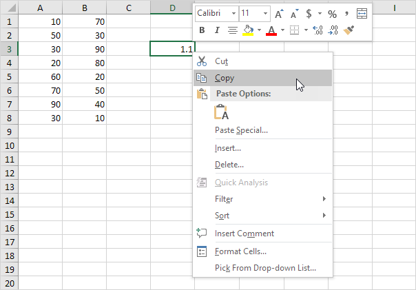


3. Select the range A1:B8.

4. Right click, and then click Paste Special.

5. Click Multiply.
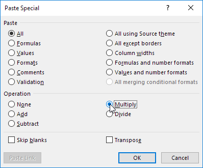


Note: you can also Divide, Add or Subtract a value.

6. Click OK.
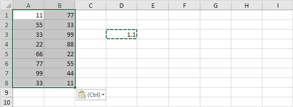


Note: all values are increased by 10 percent. Without this feature, you would have to create a temporary range (with formulas that multiply the values in the range A1:B8 by 1.1) and then replace the range A1:B8 by copy and pasting the temporary range as values.
.
Read More »

Status Bar

 The quickest way to see the average, count, numerical count, minimum, maximum or sum of selected cells is by taking a look at the status bar.

1. Select a range of cells.


2. Look at the status bar at the bottom of your window to see the sum of these cells.


3. Right click the status bar to add the average, count, numerical count, minimum or maximum.


Result:


.
Read More »

Paste Options

this article contains; Paste  |  Values  |  Formulas  |  Formatting  |  Paste Special

This example illustrates the various paste options in Excel. Cell B5 below contains the SUM function which calculates the sum of the range B2:B4. Furthermore, we changed the background color of this cell to yellow and added borders.


Paste

The Paste option pastes everything.

1. Select cell B5, right click, and then click Copy (or press CTRL + c).

2. Next, select cell F5, right click, and then click Paste under 'Paste Options:' (or press CTRL + v).


Result.


Values

The Values option pastes the result of the formula.

1. Select cell B5, right click, and then click Copy (or press CTRL + c).

2. Next, select cell D5, right click, and then click Values under 'Paste Options:'


Result.


Note: to quickly replace the formula in cell B5 with its own result, select cell B5, press F2 (to edit the formula) and press F9.

Formulas

The Formulas option only pastes the formula.

1. Select cell B5, right click, and then click Copy (or press CTRL + c).

2. Next, select cell F5, right click, and then click Formulas under 'Paste Options:'


Result.


Formatting

The Formatting option only pastes the formatting.

1. Select cell B5, right click, and then click Copy (or press CTRL + c).

2. Next, select cell D5, right click, and then click Formatting under 'Paste Options:'


Result.


Note: the Format Painter copy/pastes formatting even quicker.

Paste Special

The Paste Special dialog box offers many more paste options. To launch the Paste Special dialog box, execute the following steps.

1. Select cell B5, right click, and then click Copy (or press CTRL + c).

2. Next, select cell D5, right click, and then click Paste Special.


The Paste Special dialog box appears.


Note: here you can also find the paste options described above. You can also paste comments only, validation criteria only, use the source theme, all except borders, column widths, formulas and number formats, values and number formats. You can also use the Paste Special dialog box to perform quick operations, skip blanks and transpose data.
.
Read More »

Dynamic Named Range

 A dynamic named range expands automatically when you add a value to the range.

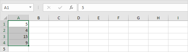
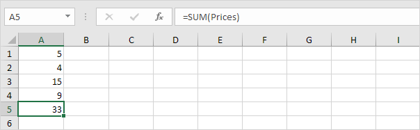
1. For example, select the range A1:A4 and name it Prices.

2. Calculate the sum.


3. When you add a value to the range, Excel does not update the sum.


To expand the named range automatically when you add a value to the range, execute the following the following steps.

4. On the Formulas tab, in the Defined Names group, click Name Manager.


5. Click Edit.


6. Click in the "Refers to" box and enter the formula =OFFSET($A$1,0,0,COUNTA($A:$A),1)


Explanation: The Offset function takes 5 arguments. Reference: $A$1, rows to offset: 0, columns to offset: 0, height: COUNTA($A:$A), width: 1. COUNTA($A:$A) counts the number of values in column A that are not empty. When you add a value to the range, COUNTA($A:$A) increases. As a result, the named range expands.

7. Click OK and Close.

8. Now, when you add a value to the range, Excel updates the sum automatically.


.
Read More »

Names in Formulas

In this article there are three main contents; Named Range  |  Named Constant  |  Name Manager

Create a named range or a named constant and use these names in your formulas. This way you can make your formulas easier to understand.
Named Range

To create a named range, execute the following steps.

1. Select the range A1:A4.


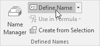
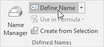
2. On the Formulas tab, in the Defined Names group, click Define Name.


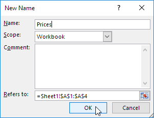
3. Enter a name and click OK.


There's an even quicker way of doing this.

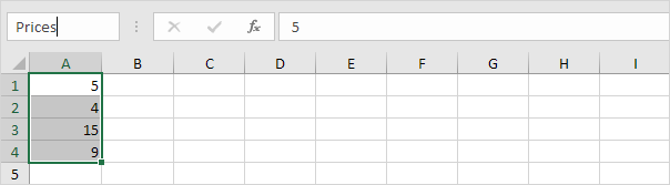
4. Select the range, type the name in the Name box and press Enter.


5. Now you can use this named range in your formulas. For example, sum Prices.


Named Constant

To create a named constant, execute the following steps.

1. On the Formulas tab, in the Defined Names group, click Define Name.


2. Enter a name, type a value, and click OK.


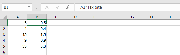
3. Now you can use this named constant in your formulas.


Note: if the tax rate changes, use the Name Manager to edit the name and Excel automatically updates all the formulas that use TaxRate.

Name Manager

To edit and delete defined names, execute the following steps.

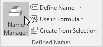
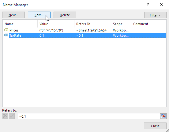
1. On the Formulas tab, in the Defined Names group, click Name Manager.


2. For example, select TaxRate and click Edit.


.
Read More »

Percent Change


The percent change formula is used very often in Excel. For example, to calculate the Monthly Change and Total Change.

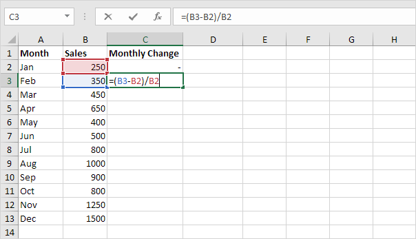
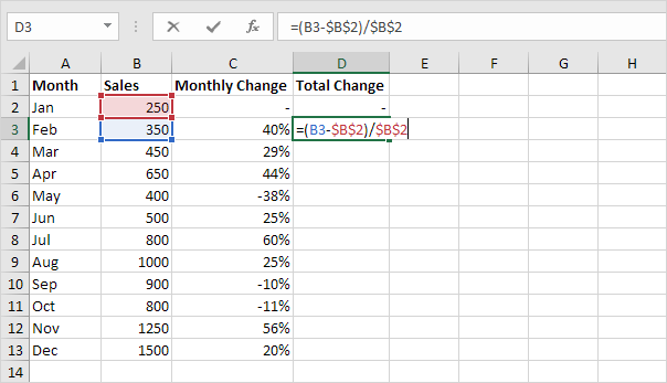
1a. Select cell C3 and enter the formula shown below.


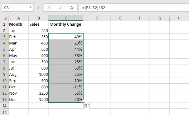
1b. Select cell C3. On the Home tab, in the Number group, apply a Percentage format.


1c. Select cell C3, click on the lower right corner of cell C3 and drag it down to cell C13.


1d. Check if everything went alright.


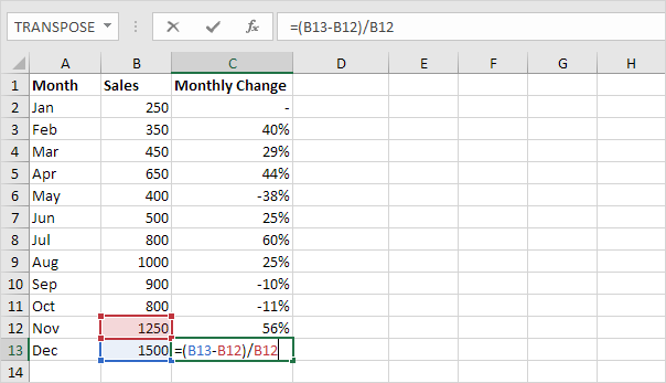
2a. In a similar way, we can calculate the Total Change. This time we fix the reference to cell B2. Select cell D3 and enter the formula shown below.


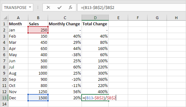
2b. Select cell D3. On the Home tab, in the Number group, apply a Percentage format.


2c. Select cell D3, click on the lower right corner of cell D3 and drag it down to cell D13.

2d. Check if everything went alright.


Explanation: when we drag the formula down, the absolute reference ($B$2) stays the same, while the relative reference (B3) changes to B4, B5, B6, etc. Maybe this is one step too far for you at this stage, but it shows you one of the many other powerful features Excel has to offer.
.
Read More »

Friday, 25 November 2016

Formulas and Functions

MS Excell is easy to calculate any thing just in seconds. you need to just enter the formula then enoy the rest part. so lets start how to find any answer. see th following figure

How to enter Formula

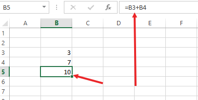
every formula is entered in formula bar as shown below,

in this bar first of all we insert = sign (Equal to) then after that we write the formula, Noe lets start the practice.


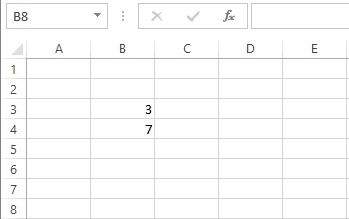
we want to add these two value, 
1. First select the Cell where you want to present the answer.
2. Then in the formula bar just type = then Location of 3 then insert + singe then location of 7,


=value+value
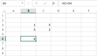
=B3+B4

then after that simple press enter and sind the answer
see below


Edit the formula

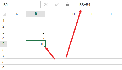
Editing the formula is also very easy. Just select the Cell in which you have enetered the formula; ANSWER CELL,  after selecting the cell see the formula bar, you will see the formula that you have enetered.


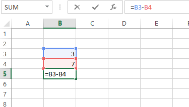
in formula bar, edit the formula according to your requirement, if you want to subract them, just change the replace the + sign wigh - sign, further detail you can watch in the video at the last of this post


Operator Precedence

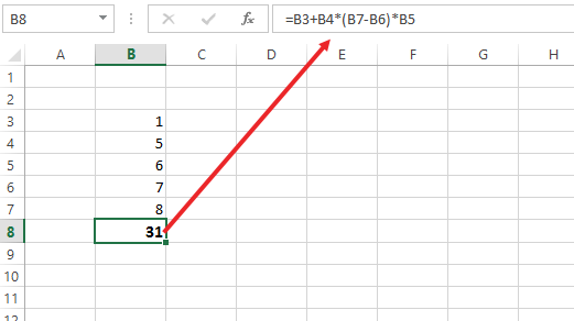
Excel uses PEMDAS rule; a default order that calculator uses. If it contains parentheses,addition multiplication and many other operation in one formula, excel calculate according to PEMDAS rule; Parentheses first and then performs multiplication or division calculations. Once this is complete, Excel will add and subtract the remainder of your formula. See the example below picture.


Copying and Pasting a Formula

When you copy a formula, MS Excel automatically adjusts the order of the formula with its cell references for each new cell the formula. To understand this, see below.

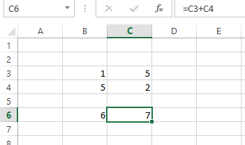
Enter the formula as you can see below into B6.


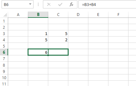
Copy a the B6 (Formula Cell)


Select cell B6, right click, and then click Copy or simple press CTRL + c to copy
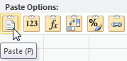
and, to past the formula, select cell C6, press CTRL + V or right click and then click Paste Option under 'Paste Options:'


or asimple you can drag the formula cell. just click the lower right dotter corner and hold and drag to C6 cell > then leave the mouse. and formula will be automatically moved to required cell where you want to paste


Result is as under


Inser the formula by Function option (Button)

Before the formula bar, you can see Function button.


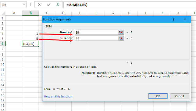
Click the cell where yuo want to show resulr (B6) then  Click on this button and you will see the following window, to add the value, just click on SUM option (shown below)


Click OK The next window will be


Now in Number 1, enter the location of first value that you want to add ie B4 and in Number 2 enter the location of second value ie B5.


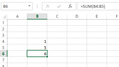
Click OK, resul is as under


this the the way about How to enter the formula, how to edit and how move/copy and paste. Now watch all this in the following Video

Read More »