Two-column Lookup

This example teaches you how to perform a two-column lookup in Excel. See the example below. We want to look up the salary of James Clark, not James Smith, not James Anderson.

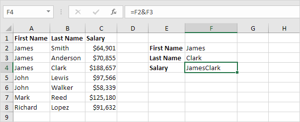
1. To join strings, use the & operator.



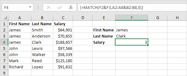
2. The MATCH function returns the position of a value in a given range. Insert the MATCH function shown below.

3. Finish by pressing CTRL + SHIFT + ENTER.



Note: The formula bar indicates that this is an array formula by enclosing it in curly braces {}. Do not type these yourself. They will disappear when you edit the formula.

Explanation: The range (array constant) A2:A8&B2:B8 is stored in Excel's memory, not in a range. The array constant looks as follows:

{"JamesSmith";"JamesAnderson";"JamesClark";"JohnLewis";"JohnWalker";"MarkReed";"RichardLopez"}

This array constant is used as an argument for the MATCH function, giving a result of 3 (JamesClark found at position 3).

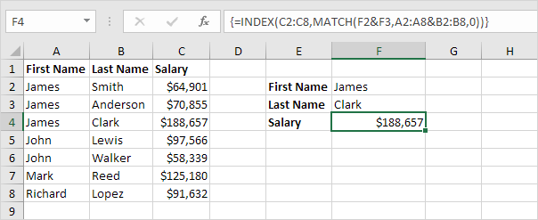
4. Use this result and the INDEX function to return the 3rd value in the range C2:C8.

.