Dependent Drop-down Lists

This example describes how to create dependent drop-down lists in Excel. Here's what we are trying to achieve:

The user selects Pizza from a drop-down list.

As a result, a second drop-down list contains the Pizza items.

To create these dependent drop-down lists, execute the following steps.

1. On the second sheet, create the following named ranges.

2. On the first sheet, select cell B1.

3. On the Data tab, click Data Validation.

The 'Data Validation' dialog box appears.

4. In the Allow box, click List.

5. Click in the Source box and type =Food.

6. Click OK.

Result:

7. Next, select cell E1.

8. In the Allow box, click List.

9. Click in the Source box and type =INDIRECT($B$1).

10. Click OK.

Result:

Explanation: the INDIRECT function returns the reference specified by a text string. For example, the user selects Chinese from the first drop-down list. =INDIRECT($B$1) returns the Chinese reference. As a result, the second drop-down lists contains the Chinese items.

.

Read More »

Drop-down List

Drop-down lists in Excel are helpful if you want to be sure that users select an item from a list, instead of typing their own values.

1. On the second sheet, type the items you want to appear in the drop-down list.

2. On the first sheet, select cell B1.

3. On the Data tab, click Data Validation.

The 'Data Validation' dialog box appears.

4. In the Allow box, click List.

5. Click in the Source box and select the range A1:A3 on Sheet2.

6. Click OK.

Result:

Tip: If you don't want users to access the items on Sheet2, you can hide Sheet2. To achieve this, right click on the sheet tab of Sheet2 and click on Hide.

7. You can also type the items directly into the text box, without using Sheet2. This gives the exact same result.

.

Read More »

Product Codes

This example teaches you how to use data validation to prevent users from entering incorrect product codes.

1. Select the range A2:A7.

2. On the Data tab, click Data Validation.

3. In the Allow list, click Custom.

4. In the Formula box, enter the formula shown below and click OK.

Explanation: this AND function has three arguments. LEFT(A2)="C" forces the user to start with the letter C. LEN(A2)=4 forces the user to enter a string with a length of 4 characters. ISNUMBER(VALUE(RIGHT(A2,3))) forces the user to end with 3 numbers. RIGHT(A2,3) extracts the 3 rightmost characters from the text string. The VALUE function converts this text string to a number. ISNUMBER checks whether this value is a number. The AND Function returns TRUE if all conditions are true. Because we selected the range A2:A7 before we clicked on Data Validation, Excel automatically copies the formula to the other cells.

5. To check this, select cell A3 and click Data Validation.

As you can see, this cell also contains the correct formula.

6. Enter an incorrect product code.

Result. Excel shows an error alert.

Note: to enter an input message and error alert message, go to the Input Message and Error Alert tab.
.

Read More »

Prevent Duplicate Entries

This example teaches you how to use data validation to prevent users from entering duplicate values.

1. Select the range A2:A20.

2. On the Data tab, click Data Validation.

3. In the Allow list, click Custom.

4. In the Formula box, enter the formula shown below and click OK.

Explanation: The COUNTIF function takes two arguments. =COUNTIF($A$2:$A$20,A2) counts the number of values in the range A2:A20 that are equal to the value in cell A2. This value may only occur once (=1) since we don't want duplicate entries. Because we selected the range A2:A20 before we clicked on Data Validation, Excel automatically copies the formula to the other cells. Notice how we created an absolute reference ($A$2:$A$20) to fix this reference.

5. To check this, select cell A3 and click Data Validation.

As you can see, this function counts the number of values in the range A2:A20 that are equal to the value in cell A3. Again, this value may only occur once (=1) since we don't want duplicate entries.

6. Enter a duplicate invoice number.

Result. Excel shows an error alert. You've already entered that invoice number.

Note: to enter an input message and error alert message, go to the Input Message and Error Alert tab.

Read More »

Budget Limit

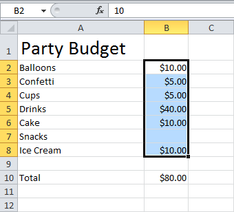
This example teaches you how to use data validation to prevent users from exceeding a budget limit.

1. Select the range B2:B8.

Note: cell B10 contains a SUM function that calculates the sum of the range B2:B8.

2. On the Data tab, click Data Validation.

3. In the Allow list, click Custom.

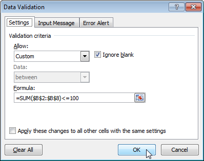
4. In the Formula box, enter the formula shown below and click OK.

Explanation: the sum of the range B2:B8 may not exceed the budget limit of $100. Therefore, we apply data validation to the range B2:B8 (not cell B10!) because this is where the values are entered. Because we selected the range B2:B8 before we clicked on Data Validation, Excel automatically copies the formula to the other cells. Notice how we created an absolute reference ($B$2:$B$8) to fix this reference.

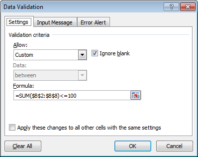
5. To check this, select cell B3 and click Data Validation.

As you can see, this cell also contains the correct formula.

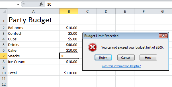
6. Enter the value 30 into cell B7.

Result. Excel shows an error alert. You cannot exceed your budget limit of $100.

Note: to enter an error alert message, go to the Error Alert tab.

Read More »

Reject Invalid Dates

This example teaches you how to use data validation to reject invalid dates.

1. Select the range A2:A4.

2. On the Data tab, click Data Validation.

Outside a Date Range

3. In the Allow list, click Date.

4. In the Data list, click between.

5. Enter the Start date and End date shown below and click OK.

Explanation: all dates between 5/20/2013 and today's date + 5 days are allowed. All dates outside this date range are rejected.

6. Enter the date 5/19/2013 into cell A2.

Result. Excel shows an error alert.

Note: to enter an input message and error alert message, go to the Input Message and Error Alert tab.

Sundays and Saturdays

3. In the Allow list, click Custom.

4. In the Formula box, enter the formula shown below and click OK.

Explanation: the WEEKDAY function returns a number from 1 (Sunday) to 7 (Saturday) representing the day of the week of a date. If a date's weekday is not equal to 1 (Sunday) AND not equal to 7 (Saturday), the date is allowed (<> means not equal to). In other words, Mondays, Tuesdays, Wednesdays, Thursdays and Fridays are allowed. Sundays and Saturdays are rejected. Because we selected the range A2:A4 before we clicked on Data Validation, Excel automatically copies the formula to the other cells.

5. To check this, select cell A3 and click Data Validation.

As you can see, this cell also contains the correct formula.

6. Enter the date 8/24/2013 (Saturday) into cell A2.

Result. Excel shows an error alert.

Note: to enter an input message and error alert message, go to the Input Message and Error Alert tab
.

Read More »

Data Validation

Use data validation in Excel to make sure that users enter certain values into a cell.

Data Validation Example

In this example, we restrict users to enter a whole number between 0 and 10.

Create Data Validation Rule

To create the data validation rule, execute the following steps.

1. Select cell C2.

2. On the Data tab, click Data Validation.

On the Settings tab:

3. In the Allow list, click Whole number.

4. In the Data list, click between.

5. Enter the Minimum and Maximum values.

Input Message

Input messages appear when the user selects the cell and tell the user what to enter.

On the Input Message tab:

1. Check 'Show input message when cell is selected'.

2. Enter a title.

3. Enter an input message.

 

Error Alert

If users ignore the input message and enter a number that is not valid, you can show them an error alert.

On the Error Alert tab:

1. Check 'Show error alert after invalid data is entered'.

2. Enter a title.

3. Enter an error message.

4. Click OK.

Data Validation Result

1. Select cell C2.

2. Try to enter a number higher than 10.

Result:

Note: to remove data validation from a cell, select the cell, on the Data tab, click Data Validation, and then click Clear All. You can use Excel's Go To Special feature to quickly select all cells with data validation.
.

Read More »