Digital World Faisalabad: Statistical Functions

MaxIfs and MinIfs

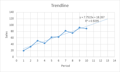
Use the MAXIFS and MINIFS function in Excel 2016 to find the maximum and minimum value based on one criteria or multiple criteria.

1. For example, the MAXIFS function below finds the highest female score.

Note: the first argument (D2:D12 in this example) is always the range in which the maximum or minimum will be determined. This MAXIFS function has 1 range/criteria pair (B2:B12/Female).

2. The MINIFS function below finds the lowest female score.

3. For example, the MAXIFS function below finds the highest female score in Canada.

Note: this MAXIFS function has 2 range/criteria pairs (B2:B12/Female and C2:C12/Canada). The MAXIFS and MINIFS function can handle up to 126 range/criteria pairs.

4. The MAXIFS function below finds the highest score below 60.

Note: this MAXIFS function only uses the range D2:D12..

Forecast and Trend

When you add a trendline to an Excel chart, Excel can display the equation in a chart (see below). You can use this equation to calculate future sales. The FORECAST and TREND function give the exact same result.

Explanation: Excel uses the method of least squares to find a line that best fits the points. The R-squared value equals 0.9295, which is a good fit. The closer to 1, the better the line fits the data.

1. Use the equation to calculate future sales.

2. Use the FORECAST function to calculate future sales.

Note: when we drag the FORECAST function down, the absolute references ($B$2:$B$11 and $A$2:$A$11) stay the same, while the relative reference (A12) changes to A13 and A14.

3. If you prefer to use an array formula, use the TREND function to calculate future sales.

Note: first, select the range E12:E14. Next, type =TREND(B2:B11,A2:A11,A12:A14). Finish by pressing CTRL + SHIFT + ENTER. The formula bar indicates that this is an array formula by enclosing it in curly braces {}. To delete this array formula, select the range E12:E14 and press Delete..

Percentiles and Quartiles

This example teaches you how to use the PERCENTILE and QUARTILE function in Excel. Below you can find a list of scores (green fill for illustration only).

1. Use the PERCENTILE function shown below to calculate the 30th percentile. Excel returns the value 12.7. This means that 30% (6 out of 20) of the scores are lower or equal to 12.7

Note: The second argument of the PERCENTILE function must be a decimal number between 0 and 1. Excel uses a slightly different algorithm to calculate percentiles and quartiles than you find in most statistics books. If you're interested, download the Excel file.

2. Use the PERCENTILE function shown below to calculate the 90th percentile. Excel returns the value 61.7. This means that 90% (18 out of 20) of the scores are lower or equal to 61.7

3. Use the QUARTILE function shown below to calculate the 1st quartile. Excel returns the value 11.25. This means that 25% (5 out of 20) of the scores are lower or equal to 11.25

Note: The second argument of the QUARTILE function must be a number between 0 and 4. PERCENTILE(A1:A20,0.25) gives the exact same result. It's up to you which function you would like to use for quartiles. Below you can find an overview.

Rank

The RANK function returns the rank of a number in a list of numbers.

1. If the third argument is omitted (or 0), Excel ranks the largest number first, second largest number second, etc.

Note: when we drag the RANK function down, the absolute reference ($A$1:$A$9) stays the same, while the relative reference (A1) changes to A2, A3, A4, etc.

2. If the third argument is 1, Excel ranks the smallest number first, second smallest number second, etc.

3. Use the RANK.AVG function to return the average rank if more than one number has the same rank.

Random Numbers

Rand | Randbetween

Excel has two useful functions when it comes to generating random numbers. The RAND and RANDBETWEEN function.

Rand

The RAND function generates a random decimal number between 0 and 1.

1. Select cell A1.

2. Type RAND() and press Enter. The RAND function takes no arguments.

3. To generate a list of random numbers, select cell A1, click on the lower right corner of cell A1 and drag it down.

Note that cell A1 has changed. That is because random numbers change every time a cell on the sheet is calculated.

4. If you don't want this, simply copy the random numbers and paste them as values.

5. Select cell C1 and look at the formula bar. This cell holds a value now and not the RAND function.

Randbetween

The RANDBETWEEN function generates a random whole number between two boundaries.

1. Select cell A1.

2. Type RANDBETWEEN(50,75) and press Enter.

3. If you want to generate random decimal numbers between 50 and 75, modify the RAND function as follows:

Negative Numbers to Zero

A clever Excel trick to change negative numbers to zero but leave positive numbers unchanged.

Below you can find two columns with numbers. To subtract the numbers in column B from the numbers in column A, execute the following steps.

1. Select cell C1.

2. Enter the formula =A1-B1

3. Click the lower right corner of cell C1 and drag the formula down.

Result:

4. To change the negative numbers to zero but leave the positive numbers unchanged, instead of =A1-B1, use =MAX(0,A1-B1) and drag the function down.

Result:

Explanation: the MAX function returns the maximum of two values. If the result of the formula is negative, the function returns 0..

Statistical Functions

Averageif

To average cells based on one criteria, use the AVERAGEIF function. For example, to calculate the average excluding zeros.

Note: < > means not equal to. The AVERAGEIF function is similar to the SUMIF function.

Median

To find the median (or middle number), use the MEDIAN function.